Computer Vision
Robot Arm, Chess Computer Vision
The game of chess is one of the world’s most popular two-player board games. I often times find myself wanting to play even when no one is around to play. One solution to this problem is to play chess on a computer or mobile device against. However, many people would agree with me in thinking that playing a virtual game of chess is a completely different experience than playing a physical game of chess. For this reason, I intend to use this project as an opportunity to build a 6 degree of freedom robotic arm that will take the place of an opponent in a physical game of Chess. The state of the game will be determined by applying chess computer vision algorithms to images from a camera that will be mounted above the game board facing down.
The Setup
Chessboard
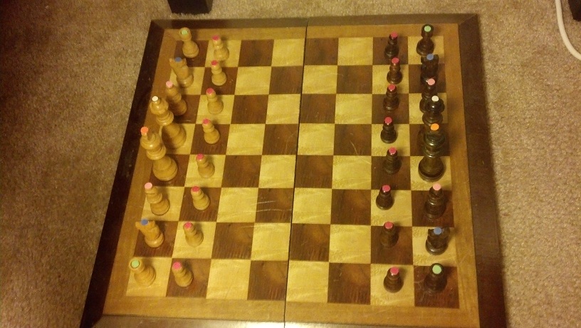
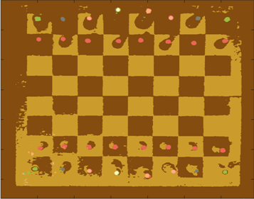
The chessboard used for this project is a standard wood chess board with 64 tiles, and 32 pieces.
The Robot Arm
I designed a 3R spatial manipulator in Autodesk Inventor 2013 and constructed the arm out of medium density fiber board. The joints are controlled by 7 servos connected to an Arduino microcontroller. I wrote a simple program for the Arduino that processes incoming serial commands that tell it joint positions in degrees.
Arm Design in Inventor

Autodesk Inventor design of a 3R 6DOF robot arm manipulator

MDF Constructed 3R Robot Arm
Camera Calibration
I calibrated by personal webcam for this project. The MATLAB Camera Calibration Toolbox was used to determine the intrinsic calibration parameters of my camera. I was surprised to find that my camera has very little radial distortion.
Distortion Example
The web cam introduces very little radial distortion, as can be seen by the images below
|
Distorted Image from Webcam |
After Undistortion |
 |
 |
Chess Computer Vision
My low target for this project is to identify the chessboard. I have managed to detect a calibration chessboard, and a real chess board. I did a little math to find the centers of the tiles which will be my starting point for determining if a piece is occupying the tile. For detecting the board I made use of libcbdetect.
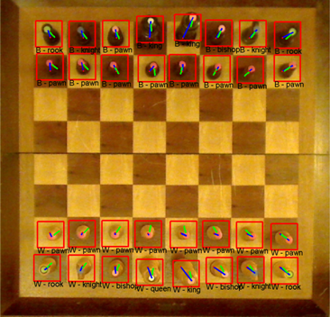
Examples of Detected Chessboards
In these examples, the chess board has been identified and the centers of the tiles have been marked.
|
Black and White Calibration Chess Board |
Real Chess Board |
 |
 |
Potential Problem – Height of Chess Pieces and Perspective
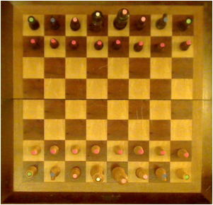
One problem I ran into is that the height of some the Chess pieces causes the colored markers to appear outside of the tiles that the piece is in. This is due to the camera’s perspective on the scene. I reduced the extent of this problem by increasing the camera’s distance from the board.
Finding the Pieces
In order to identify the pieces from the top-down perspective provided by the camera, I attached colored pieces of paper to the top of each chess piece. In chess, each of the two players begins with 16 pieces, spanning 6 different classes. I assigned each of the 6 classes a unique color and attached hole-punched pieces of paper to the tops of each piece. The color of the piece of paper is used to determine the class of piece, while the color of the piece is used to determine if the piece belongs to player 1 or player 2.
The pieces are mapped to colors as follows:
| Chess Piece | Color |
| Pawn | Red |
| Rook | Green |
| Knight | Blue |
| Bishop | Pink |
| Queen | White |
| King | Orange |
LAB Color Space
In order to effectively discriminate color, I had to find a color space that lent itself to this. I found that the LAB color space is common for color discrimination because it is more perceptually linear than other color spaces. To test its discriminative qualities for the purposes of this project, I took a few color samples of the potential colors for chess pieces and plotted them in LAB space. Here are three slices of the LAB space with varying L-values:

Here is a 3D plot of the color samples:
Color Identification
Color identification turned out to be quite a bit more difficult that I originally thought it would be. The variations in lighting caused a significant amount of variance in the detected colors. In order to capture the variance of the colors due to small variations in lighting I fitted color samples to Gaussian mixture models.
For each color, I collected samples of the color from images of the board with varying illumination and fitted the samples to a 3D Gaussian mixture model. Here is a depiction of the fitted Gaussians in LAB space. Each color is represented by a single Gaussian.
Segmenting Images by Color
In order to separate pieces from the board, I segmented the images based on pixel colors. To segment the image, I begin by converting an input image to the LAB color space. Then, for each pixel in the image, I compute the Mahalanobis distance from the pixel to each color’s Gaussian mixture model representation. I then find nearest Gaussian to the pixel and map the pixel to the color represented by said Gaussian.
Example Segmentation
| Input Image | Segmented Image |
 |
 |
From this point, I can easily isolate specific colors from the image.
Connected Component Blobs
Once the image is segmented, I calculate a binary mask that represents the locations of all of the chess pieces. I then perform morphological closing and opening to clean up the image and remove noisy color segmentation. Continuing with the output from the color segmentation above, here is the resulting binary mask of chess pieces:
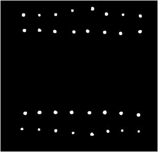
This example contains perfect segmentation, but this isn’t always possible. For example, here is a noisy segmentation:
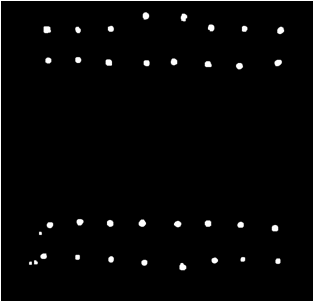
Usually noise results in blobs that are smaller than the actual chess pieces, so I remedied this problem by processing the blobs in order of decreasing size.
Identifying Pieces
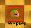
To determine the class of piece for each blob detection I pull the index of the color of the isolated blob from the segmented image. Once the class of piece is detected, I must detect which players piece it is; black or white. Determining if the piece is black or white is accomplished by analyzing color samples along a line from the centroid of the blob to the center of the chess board. I only collect samples that are right outside the edge of the color blob, because this is the location where black or white pixels are.
For example, here is a detected white pawn. The blue line represents the offset from the center of the detected blob to the tile center. The green line represents the locations where color samples were collected for determining if the piece is white or black.
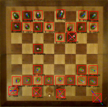
Here are examples of chess piece classification. From the images below, it is clear that variations in lighting cause problems for the classification process. I may be able to build a more robust model for representing the colors by using more color samples across a wider range of illuminations. It may be worthwhile to consider using Gaussian mixture models with more mixture components per color.
Correct Classification:
Incorrect Classification:
Problems
Here are some of the problems I ran into during this project.
- Variations in Lighting
- Possible Solutions:
- Use more diverse color samples for GMM’s
- Use multiple Gaussians per color
- Possible Solutions:
- Real-time
- Webcam auto adjustments (focus, lighting)
- Chess board & Pieces
- Glossy finish causes color misclassification
Eye Tracking via Webcam
The mouse has undoubtedly become an integral part of personal computing as we know it. Be it a laptop or a desktop, it seems no workstation is complete without a keyboard and mouse. But just how efficient is it to use a mouse to control a cursor? What if you could control your mouse cursor with just your eyes? You would never have to take your right hand (or left) off the keyboard! It’s a simple idea, and it makes sense.
When moving the cursor, I’ve noticed that people usually do one of two things:
- They follow the cursor with their eyes until it reaches the intended destination (where they want to click), or
- They look at the intended destination (where they want to click) and wait for their hand to get the cursor there.
I’d say #2 is more common among frequent computer users, but either way, there is a delay between deciding what to click and actually getting the cursor there to click it. The summation of this lag time certainly adds up. I’d have to do a little more thinking to come up with a rough estimate of just how much time could be saved, but this isn’t my motivation. My motivation is the fact that this is just a really cool and inexpensive-to-test idea.
The Idea
So anyway, the idea is to be able to determine where exactly on the screen the user is looking just by examining the position of the eyes (as seen from a webcam). But what about clicks? Well, click events could be triggered by many things; maybe a quick head nod, an emphatic blink, or simply a dedicated key on the keyboard. There are many possible solutions for triggering left/right/middle mouse clicks. I’ll just have to try out various methods and see which ones work the best.
Source: Unknown
A simple Google search will show that extensive research has already been done on the topic of eye tracking. However, it seems that modern approaches require the user to wear some sort of head gear to track eye movement. This can be costly, inconvenient, and likely requires a less-than-trivial amount of calibration –The exact opposite of the convenience that humans naturally seek.
This idea may be better suited for laptops than desktops, because majority of laptops today have built in webcams. Webcams that can’t move relative to the screen. This means extrinsic camera calibration would only need to be performed once per laptop. However, with standalone webcams (commonly used with desktop computers) it may be necessary to recalibrate every time the webcam is moved -or even bumped for that matter.
Applications
Aside from the convenience of being able to move a cursor with just your eyes, this technology has potential for many applications. One of which is analyzing what us humans spend the most time looking at when shown pictures, videos, or text. A heat map can be generated to represent areas of an image (or a website) that someone is most interested in. This has been done in many variations in the past, but providing a way for this analysis to be performed by consenting users in the comfort of their own homes (without fancy headgear) could certainly lead to an expansion in this field of research.
Conclusion
I still need to do more research on the topic. I may find that the required precision/accuracy needed for effectively controlling a mouse cursor with eye-movement alone is beyond the reach of current webcams.
Interesting Notes
- I may also be able to determine how close a user is sitting to the computer monitor (within a reasonable degree of error). This can be calculated as the height of the triangle formed by two eyes and a point of interest on screen. Assuming, of course, that the user is focusing on point that lies on the plane defined by the computer screen.
Projective Chirp

- (a) In image processing, direct periodicity seldom occurs, but, rather, periodicity-in-perspective is encountered.
- (b) Repeating structures like the alternating dark space inside the windows, and light space of the white concrete, “chirp” (increase in frequency) towards the right.
- (c) Thus the best fit chirp for image processing is often a projective chirp.
Full Article: http://en.wikipedia.org/wiki/Chirp
Line Detection via Hough Transform
I’ve had a hard time finding an explanation for how exactly hough transform works. No one seemed to key-in on a detail that was most integral to my understanding. So I will explain hough transform briefly while emphasizing the detail that helped me understand the Hough Transform.
The Hough Transform
First, begin with an image that you want to find lines in. I chose an image of a building for this example.

Then run your favorite edge detection algorithm on it. I chose canny edge detection.

Note: The lines are aliased here… and yes, as you might suspect, it does sometimes cause problems. But there is a simple way to handle it. Just increase the bin size for the accumulator matrix.
Note2: If you (..yes, you!) would like to know more about how aliased lines cause problems, just say so in the comments and I’ll do my best to shed light on the issue 😉
How to Generate a Hough Transform Accumulator Matrix
This is the important part. The edge map (above) is what is used to generate the Hough accumulator matrix.
Okay. Here’s the trick… Each white pixel in the edge map will create a one pixel sine wave in the Hough accumulator matrix.
That means.. 1 pixel in edge map = 1 sine wave in accumulator matrix.
Use the [x,y] coordinates of white pixels in the edge map as parameters for computing [ρ, θ] needed for the sine wave that will go into the accumulator matrix.
The general equation is: ρ = x*cos(θ) + y*sin(θ)
So for each white pixel, loop from θ = –90 to θ = 90, calculating ρ at each iteration.
For each [ρ, θ] pair, the accumulator matrix gets increased by 1.
That is: AccumulatorMatrix[θ, ρ] = AccumulatorMatrix[θ, ρ] + 1;
The Hough Transform Accumulator Matrix
So now we’ve done it. We’ve accumulated sine waves for each white pixel in the edge map. Now all we need to do is extract the useful information out of it!
")
This is essentially a grayscale image depicted with a JET colormap, so don’t worry if yours doesn’t look quite like this. You’ll know you did something wrong if you don’t see any sinusoidal lines. (You may need to scale your image linearly to bring out the detail.)
How to get Lines from the Accumulator Matrix
The first thing you do is threshold the accumulator matrix to find the hot spots in the image. The [x,y] coordinates of each hot spot define a point in a polar coordinate system. A point in the polar coordinate system is defined by ρ (rho, length) and θ (theta, angle). In this example, I believe I used a bin size of 1 when I filled the accumulator matrix. This means the polar variables ρ = y, and θ = x. If you’re using a bin size other than one, just scale the values, ρ = y*binSize, θ = x*binSize.
Once you have a polar point, imagine a vector from the origin to that polar point, the line that is detected in the image is perpendicular to that vector, and crosses through that point.
The value of the hotspot in the accumulator matrix is the number of pixels from the edge map that lie on that line.
The Result

I plotted 14 (of the many) lines that were detected based on the above hough transform. I could have extracted more lines from the image by changing the value I thresholded the accumulator matrix with. If I would’ve chosen a lower threshold value, more lines would have been detected.
Questions, Comments, Concerns?