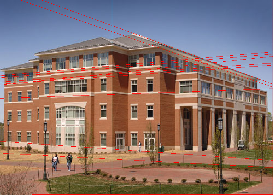
line detection
Line Detection via Hough Transform
I’ve had a hard time finding an explanation for how exactly hough transform works. No one seemed to key-in on a detail that was most integral to my understanding. So I will explain hough transform briefly while emphasizing the detail that helped me understand the Hough Transform.
The Hough Transform
First, begin with an image that you want to find lines in. I chose an image of a building for this example.
Then run your favorite edge detection algorithm on it. I chose canny edge detection.
Note: The lines are aliased here… and yes, as you might suspect, it does sometimes cause problems. But there is a simple way to handle it. Just increase the bin size for the accumulator matrix.
Note2: If you (..yes, you!) would like to know more about how aliased lines cause problems, just say so in the comments and I’ll do my best to shed light on the issue 😉
How to Generate a Hough Transform Accumulator Matrix
This is the important part. The edge map (above) is what is used to generate the Hough accumulator matrix.
Okay. Here’s the trick… Each white pixel in the edge map will create a one pixel sine wave in the Hough accumulator matrix.
That means.. 1 pixel in edge map = 1 sine wave in accumulator matrix.
Use the [x,y] coordinates of white pixels in the edge map as parameters for computing [ρ, θ] needed for the sine wave that will go into the accumulator matrix.
The general equation is: ρ = x*cos(θ) + y*sin(θ)
So for each white pixel, loop from θ = –90 to θ = 90, calculating ρ at each iteration.
For each [ρ, θ] pair, the accumulator matrix gets increased by 1.
That is: AccumulatorMatrix[θ, ρ] = AccumulatorMatrix[θ, ρ] + 1;
The Hough Transform Accumulator Matrix
So now we’ve done it. We’ve accumulated sine waves for each white pixel in the edge map. Now all we need to do is extract the useful information out of it!
This is essentially a grayscale image depicted with a JET colormap, so don’t worry if yours doesn’t look quite like this. You’ll know you did something wrong if you don’t see any sinusoidal lines. (You may need to scale your image linearly to bring out the detail.)
How to get Lines from the Accumulator Matrix
The first thing you do is threshold the accumulator matrix to find the hot spots in the image. The [x,y] coordinates of each hot spot define a point in a polar coordinate system. A point in the polar coordinate system is defined by ρ (rho, length) and θ (theta, angle). In this example, I believe I used a bin size of 1 when I filled the accumulator matrix. This means the polar variables ρ = y, and θ = x. If you’re using a bin size other than one, just scale the values, ρ = y*binSize, θ = x*binSize.
Once you have a polar point, imagine a vector from the origin to that polar point, the line that is detected in the image is perpendicular to that vector, and crosses through that point.
The value of the hotspot in the accumulator matrix is the number of pixels from the edge map that lie on that line.
The Result
I plotted 14 (of the many) lines that were detected based on the above hough transform. I could have extracted more lines from the image by changing the value I thresholded the accumulator matrix with. If I would’ve chosen a lower threshold value, more lines would have been detected.
Questions, Comments, Concerns?


