Music Theory Basics
Came across a few things while reading about music theory today and thought it might be useful to keep track of some of the basics. …So here goes..
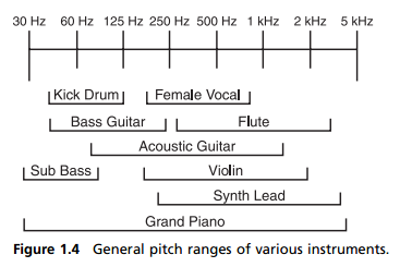
General Pitch Ranges of Various Instruments
Thought it might come in handy later for equalizer config.
Synthesis
In additive synthesis, the required waveform is obtained by adding harmonic waves to a given fundamental. The reverse of this process is called subtractive synthesis. Subtractive synthesis behinds with a waveform rich in harmonic content and then selectively filters out certain frequencies.
The oscillator produces sound in a synthesizer. The oscillator is capable of producing both frequency and harmonic content.
- Sine wave – composed on only one specific frequency.
- Square wave – emphasizes odd-numbered harmonics. Produces a hollow sound. Works well for basses.
- Triangluar wave – emphasizes few specific odd-numbered partials. Produces a clear note, good for imitating sounds of flutes.
- Sawtooth wave – rich in harmonics. Used to imitate string and brass sounds. Common in trance style rich lead synths.
Properties of Sound
Sound Envelope – The way in which a sound develops over time. There are four components: attack, decay, sustain, and release:
- Attack time – time taken for a sound to reach a (maximum) level of loudness.
- Sustain time – time sound remains at a constant level (often maximal).
- Decay time – time taken for sound to fall from sustained loudness to zero loudness.
- Attack / Sustain / Decay defines a sound envelope.
Timbre – created by the kind and number of overtones.
- The tone heard as pitch is called the fundamental tone or the first harmonic of a sound.
- Overtones are additional tones of higher pitch than, and superposed over, the fundamental tone.
- Rich, full sounds (violin, voice) have many overtones, pure, thin sounds (flute, triangle) have few overtones.
Average Tempo Based on Type of Music
- Ambient – 50-100 BPM
- Hip-hop – 70-95 BPM
- Deep House – 110-130 BPM
- Trance – 130-145 BPM
- Hard dance / hardcore – 145-170 BPM
- Drum and bass – 160-180 BPM
Scales
W = Whole step (whole tone), H = Half step (semi-tone)
Major Scale: w-w-h-w-w-w-h (ex. C,D,E,F,G,A,B,C)
Minor Scale: w-h-w-w-h-w-w (ex. A,B,C,D,E,F,G,A)
Note Intervals
The note intervals from 1-12 half-steps:
- minor second
- major second
- minor third
- major third
- perfect fourth
- Diminished fifth
- Perfect fifth
- minor sixth
- major sixth
- minor seventh
- major seventh
- octave
Intervals large than an octave are called compound intervals. This is because they represent a simple interval (12 or less half-steps) plus one or more octaves. For example, an eleventh is also called a compound fourth. To calculate what notes are used in a compound interval, simple take the number, for example, a twentyfourth interval is simply (24 mod 7 = 3) a compound third.
Things to check out
- psychoacoustics – The study of the way in which we hear and perceive sound vibrations.
Java Socket Server – Clients Disconnecting (Ungracefully)
If you’re writing a java socket server you’ll need to detect when a client disconnects — even if they don’t have the courtesy to disconnect gracefully. This is especially annoying if you’re sending the client socket a lot of streaming data and the client just stops listening without saying a word.
If you’re using an PrintStream to write data to the socket, the way to check this is to check the result from PrintStream.checkError(). If its false, the client disconnected. I’m assuming other output streams will have similar functionality.
If the client doesn’t disconnect gracefully, these things may still occur:
- Socket.isConnected() may return true
- Socket.isClosed() may return return false
- Socket.isInputShutdown() may return false
- Socket.isOutputShutdown() may return false
I just wasted an hour figuring this out.. Hopefully it will help someone.
Line Detection via Hough Transform
I’ve had a hard time finding an explanation for how exactly hough transform works. No one seemed to key-in on a detail that was most integral to my understanding. So I will explain hough transform briefly while emphasizing the detail that helped me understand the Hough Transform.
The Hough Transform
First, begin with an image that you want to find lines in. I chose an image of a building for this example.
Then run your favorite edge detection algorithm on it. I chose canny edge detection.
Note: The lines are aliased here… and yes, as you might suspect, it does sometimes cause problems. But there is a simple way to handle it. Just increase the bin size for the accumulator matrix.
Note2: If you (..yes, you!) would like to know more about how aliased lines cause problems, just say so in the comments and I’ll do my best to shed light on the issue 😉
How to Generate a Hough Transform Accumulator Matrix
This is the important part. The edge map (above) is what is used to generate the Hough accumulator matrix.
Okay. Here’s the trick… Each white pixel in the edge map will create a one pixel sine wave in the Hough accumulator matrix.
That means.. 1 pixel in edge map = 1 sine wave in accumulator matrix.
Use the [x,y] coordinates of white pixels in the edge map as parameters for computing [ρ, θ] needed for the sine wave that will go into the accumulator matrix.
The general equation is: ρ = x*cos(θ) + y*sin(θ)
So for each white pixel, loop from θ = –90 to θ = 90, calculating ρ at each iteration.
For each [ρ, θ] pair, the accumulator matrix gets increased by 1.
That is: AccumulatorMatrix[θ, ρ] = AccumulatorMatrix[θ, ρ] + 1;
The Hough Transform Accumulator Matrix
So now we’ve done it. We’ve accumulated sine waves for each white pixel in the edge map. Now all we need to do is extract the useful information out of it!
This is essentially a grayscale image depicted with a JET colormap, so don’t worry if yours doesn’t look quite like this. You’ll know you did something wrong if you don’t see any sinusoidal lines. (You may need to scale your image linearly to bring out the detail.)
How to get Lines from the Accumulator Matrix
The first thing you do is threshold the accumulator matrix to find the hot spots in the image. The [x,y] coordinates of each hot spot define a point in a polar coordinate system. A point in the polar coordinate system is defined by ρ (rho, length) and θ (theta, angle). In this example, I believe I used a bin size of 1 when I filled the accumulator matrix. This means the polar variables ρ = y, and θ = x. If you’re using a bin size other than one, just scale the values, ρ = y*binSize, θ = x*binSize.
Once you have a polar point, imagine a vector from the origin to that polar point, the line that is detected in the image is perpendicular to that vector, and crosses through that point.
The value of the hotspot in the accumulator matrix is the number of pixels from the edge map that lie on that line.
The Result
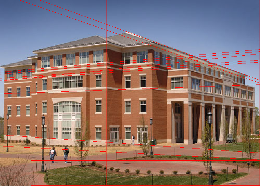
I plotted 14 (of the many) lines that were detected based on the above hough transform. I could have extracted more lines from the image by changing the value I thresholded the accumulator matrix with. If I would’ve chosen a lower threshold value, more lines would have been detected.
Questions, Comments, Concerns?


